Tracking by Predicting 3-D Gaussians Over Time

doi:10.48550/arXiv.2512.22489

Video-GMAE

Tracking by Predicting 3-D Gaussians Over Time

Zero-shot tracking emerges from 3-D Gaussian motion.

view_in_ar Gaussian video tokens

Represent each clip with a fixed set of 3-D Gaussians that move in time, matching the 2-D projection of a dynamic 3-D scene.

link Correspondence by construction

Predict per-Gaussian deltas (translation + color) per frame so identities persist; reconstruction loss enforces temporal consistency.

center_focus_strong Tracking emerges

Project Gaussian trajectories to the image plane to obtain zero-shot point tracking; light fine-tuning yields further gains.

description Paper (PDF) library_books Supplementary movie Videos (ZIP) code Code article arXiv

Method

Masked video → ViT encoder → Gaussians for frame 1 + deltas for later frames → differentiable splatting reconstruction.

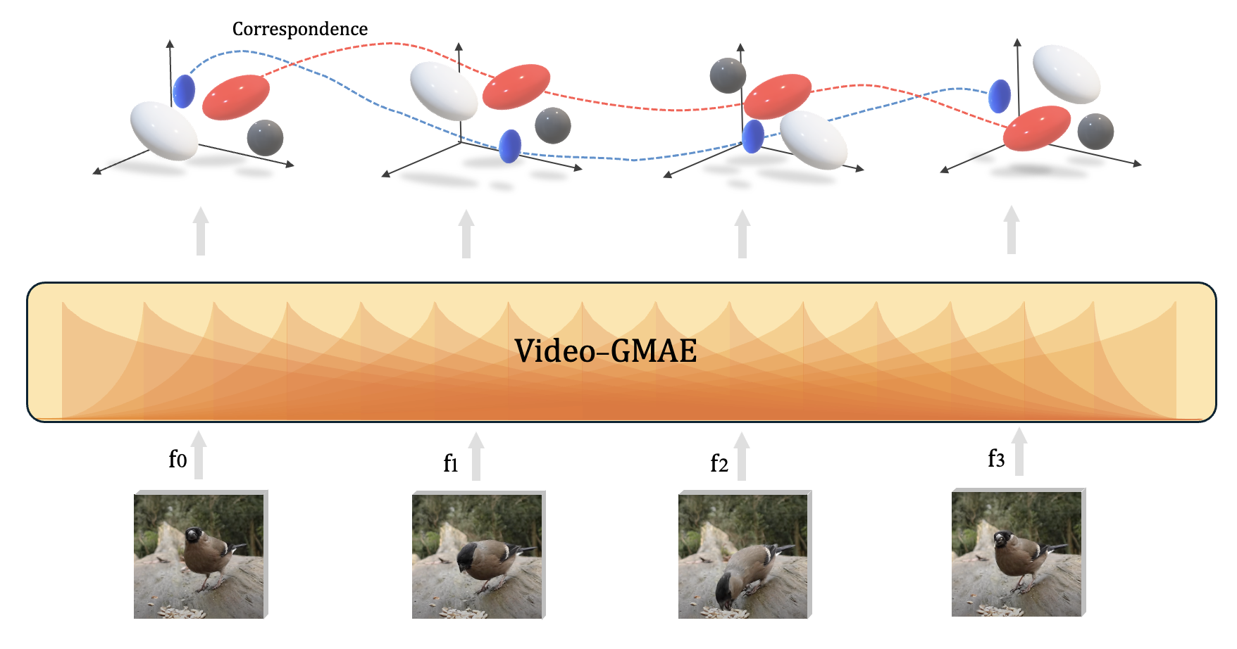
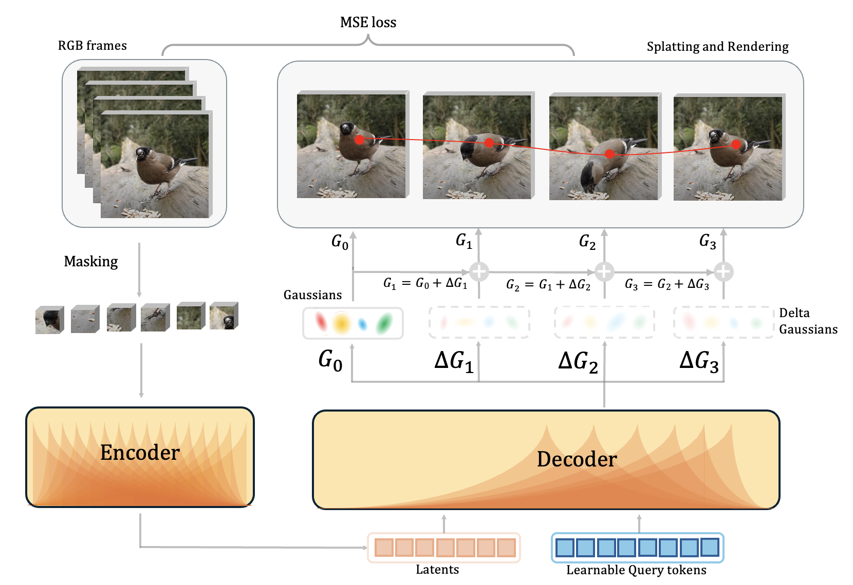Pretraining pipeline with Gaussian splatting — Video masked autoencoding via Gaussian splatting.

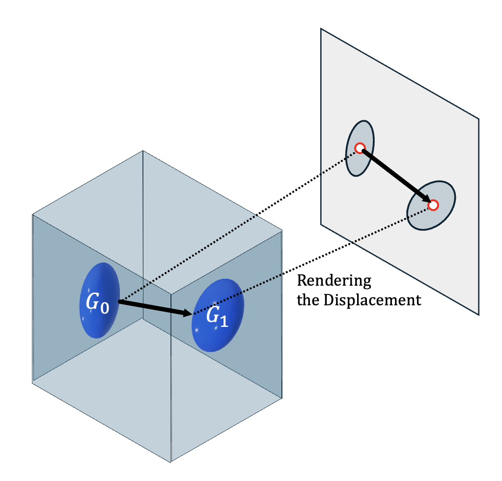Zero-shot tracking schematic — Projecting Gaussian motion to image-plane flow for zero-shot tracking.

Zero-shot tracking recipe (details)

Render Gaussian motion as dense flow, then advect points.

Predict Gaussian motion per frame.
Project Gaussians to image-plane flow.
Advect query points with the flow.
Use anchor Gaussians when occluded (optional).

Projected centers: \(x_i^{(t)} = \Pi(\mu_i^{(t)})\)

Displacement: \(\Delta x_i^{(t)} = x_i^{(t+1)} - x_i^{(t)}\)

Flow: \(F^{(t)}(u) = \sum_i \alpha_i^{(t)}(u)\,\Delta x_i^{(t)}\)

Update: \(p^{(t+1)} = p^{(t)} + F^{(t)}(p^{(t)})\)

Occlusion-aware variant

Keep a fixed top‑k anchor set from the first frame, track their visibility, and mix flow with anchor proposals when visible mass is low.

Anchor mass: \(\omega^{(t)} = \sum_{i\in\mathcal{S}} \alpha_i^{(t)}(p^{(t)})\)

Weights over anchors: \(\tilde{\pi}_i^{(t)} = \dfrac{\alpha_i^{(t)}(p^{(t)})}{\sum_{j\in\mathcal{S}} \alpha_j^{(t)}(p^{(t)}) + \varepsilon}\)

Anchor proposal: \(\hat{p}_{\text{anch}}^{(t+1)} = \sum_{i\in\mathcal{S}} \tilde{\pi}_i^{(t)} \left(x_i^{(t)} + \Delta x_i^{(t+1)}\right)\)

Blend with flow if visible: \(p^{(t+1)} = (1-\beta)\big(p^{(t)} + F^{(t)}(p^{(t)})\big) + \beta\,\hat{p}_{\text{anch}}^{(t+1)}\)

Otherwise use anchors only: \(p^{(t+1)} = \hat{p}_{\text{anch}}^{(t+1)}\)

Hyperparams (from paper): k = 8, \(\tau_{\text{vis}} = 0.5\), \(\beta = 0.3\).

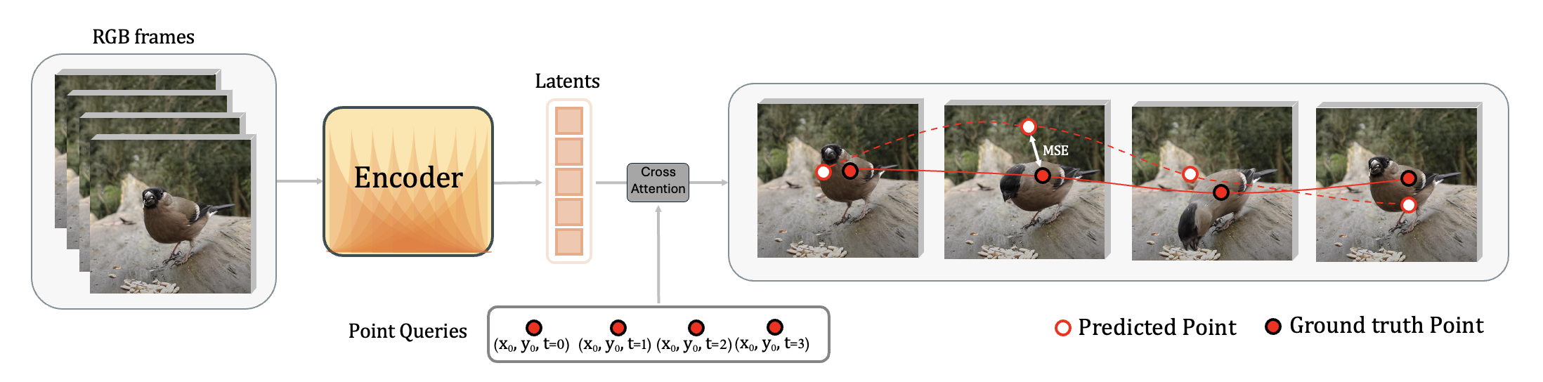Fine-tuning cross-attention readout — Fine-tuning: cross-attention readout over encoder latents improves precision and occlusion handling.

Pretraining

High masking ratio; decoder predicts Gaussians for frame 1 plus per-frame deltas; splatting closes the loop.

Zero-shot tracking

Project Gaussian motion to a flow field and advect points—no tracking labels.

Fine-tuning

Cross-attention readout over encoder latents sharpens localization and occlusion handling.

Results

From zero-shot tracking to fine-tuned precision; videos are the primary evidence.

Zero-shot

Stable tracks emerge from Gaussian motion without labels.

Jump to zero-shot

Comparisons

Video-GMAE vs. GMRW‑C: stability vs. tiny-detail fidelity.

See comparisons

Fine-tuned

Light supervision sharpens trajectories and occlusion handling.

View fine-tuned

Reconstructions

Pretraining renders show what the Gaussians capture.

Watch recon

Zero-shot Tracking

Correspondence emerges directly from Gaussian motion—no tracking labels.

What to look for:

DAVIS: deforming objects and occlusions.
Kinetics: diverse human actions and interactions.
Failure modes: camera motion + high-frequency backgrounds + 256-Gaussian budget.

DAVIS zero-shot.

Kinetics zero-shot.

Zero-shot failure cases.

Comparisons vs. GMRW‑C

Video-GMAE is more temporally stable; GMRW‑C can better preserve tiny, fast details.

What to look for:

Stability vs. early occlusion/dropouts.
Tiny fast parts where GMRW‑C may track tighter.

TAP-Vid Kinetics comparison.

TAP-Vid DAVIS comparison.

Fine-tuned Tracking

Light supervision sharpens localization and occlusion handling.

What to look for:

Reduced drift/jitter vs. zero-shot.
More reliable occlusion handling.

Fine-tuned: TAP-Vid DAVIS (two sequences, looped).

Fine-tuned: TAP-Vid Kinetics (two sequences, looped).

Pretraining Reconstructions

Rendered Gaussian trajectories during pretraining capture coarse structure and motion.

What to look for:

Coarse geometry and motion with few Gaussians.
Fine detail limited by the 256-Gaussian budget.

Dynamic reconstructions from Gaussians.

Quantitative Results

Bars below show Video-GMAE zero-shot gains over GMRW on Kinetics and Kubric.

Kinetics vs. GMRW +34.6%

Kubric vs. GMRW +13.1%

DAVIS vs. GMRW -1.2%

Limitations

Static-camera assumption in pretraining can hurt videos with strong camera motion.
256-Gaussian budget limits fine-detail fidelity in busy scenes.
Longer-frame correspondence regularization can degrade learning on very long horizons.

BibTeX

Cite this work as arXiv:2512.22489.

@misc{baranwal2025tracking3d,
  title         = {Tracking by Predicting 3-D Gaussians Over Time},
  author        = {Tanish Baranwal and Himanshu Gaurav Singh and Jathushan Rajasegaran and Jitendra Malik},
  year          = {2025},
  eprint        = {2512.22489},
  archivePrefix = {arXiv},
  primaryClass  = {cs.CV},
  doi           = {10.48550/arXiv.2512.22489},
  url           = {https://arxiv.org/abs/2512.22489}
}