Tracking by Predicting 3-D Gaussians Over Time

Baranwal, Tanish; Singh, Himanshu Gaurav; Rajasegaran, Jathushan; Malik, Jitendra

Video-GMAE Point tracking from Gaussian motion

Tracking by Predicting3-D Gaussians Over Time

Tanish Baranwal Himanshu Gaurav Singh Jathushan Rajasegaran Jitendra Malik

Tracking emerges for free.

A masked autoencoder learns video as moving 3-D Gaussians, and a point tracker falls out with zero tracking labels.

Zero-shot tracks from Gaussian motion on DAVIS.

95%masked video tokens

16frames per clip

256Gaussians per frame

0tracking labels

Kinetics · Kubric · DAVISunlabeled pretraining video

description Paper library_books Supplementary movie Videos code Code article arXiv

01 The idea

Video as moving 3-D Gaussians

Each primitive keeps its identity

Motion is residual ΔG, so a Gaussian at frame t is the same Gaussian at t+1.

Correspondence as a 3-D prior

Encoding video as moving Gaussians makes the SSL task harder and pushes latents toward long-range correspondence.

Only part of each primitive moves

The 3-D mean μ and color r receive per-frame residuals; scale, rotation, and opacity stay fixed.

02 Method pipeline

Pretrain, read out, fine-tune

Pretraining pipeline with Gaussian splatting — Video masked autoencoding through Gaussian splatting: the decoder predicts a moving Gaussian scene, then reconstruction closes the loop.

Zero-shot tracking schematic — Render Gaussian displacement into image-plane flow, then advect query points.

Zero-shot trackno labels · no flow · no boxes

Project\(x_i^{(t)} = \Pi(K[R|t], \mu_i^{(t)})\)

Displace\(\Delta x_i^{(t+1)} = x_i^{(t+1)} - x_i^{(t)}\)

Render flow\(F^{(t)}(u) = \sum_{i=1}^{n}\alpha_i^{(t)}(u)\cdot\Delta x_i^{(t)}\)

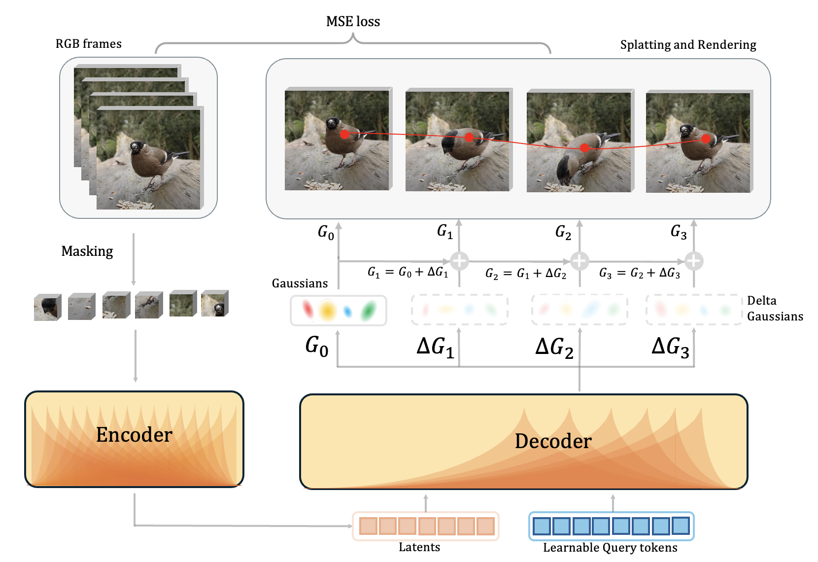
1Predict Gaussian means through time with \(\mu_i^{(t+1)}=\mu_i^{(t)}+\Delta\mu_i^{(t)}\), then project the same primitives at adjacent frames into image coordinates.
2Replace each Gaussian's color with its 2-D displacement \((\Delta x_{i,x}^{(t)}, \Delta x_{i,y}^{(t)}, 0)\) and splat those values with the renderer's opacity weights to obtain dense flow \(F^{(t)}\).
3For each query point, bilinearly sample flow and opacity at \(p^{(t)}\). The pure flow proposal is \(a^{(t)}=p^{(t)}+F^{(t)}(p^{(t)})\).
4Fix a top-k anchor set \(\mathcal{S}\) from frame 0, compute anchor mass \(\omega^{(t)}=\sum_{i\in\mathcal{S}}\alpha_i^{(t)}(p^{(t)})\), and renormalize anchor weights \(\tilde{\pi}_i^{(t)}\).
5Use the anchor proposal \(s^{(t+1)}=\sum_{i\in\mathcal{S}}\tilde{\pi}_i^{(t)}(x_i^{(t)}+\Delta x_i^{(t+1)})\) to preserve identity around occlusion.
6If \(\omega^{(t)}\ge\tau_{\mathrm{vis}}\), update \(p^{(t+1)}=(1-\beta)a^{(t)}+\beta s^{(t+1)}\) and mark visible; otherwise set \(p^{(t+1)}=s^{(t+1)}\) and mark occluded.

k = 8τ_vis = 0.5β = 0.3

Fine-tuning cross-attention readout — Fine-tuning adds a supervised cross-attention readout over frozen or trainable encoder latents to sharpen localization and occlusion handling.

03 Results map

Coherent across motion and occlusion

Zero-shot tracks emerge directly from Gaussian motion, and light supervision sharpens the readout.

Zero-shot

No labels, no flow, no boxes

Stable tracks emerge directly from Gaussian motion.

Watch zero-shot

Comparisons

Stable over time

Video-GMAE tends to preserve temporal coherence; GMRW-C can keep tiny fast details tighter.

Compare methods

Fine-tuned

Supervised readout

Kubric labels sharpen trajectories and occlusion handling.

View fine-tuned

Reconstructions

What the Gaussians capture

Rendered pretraining outputs show coarse structure, motion, and the limits of the Gaussian budget.

Watch recon

04 Tracks across benchmarks

Zero-shot tracking

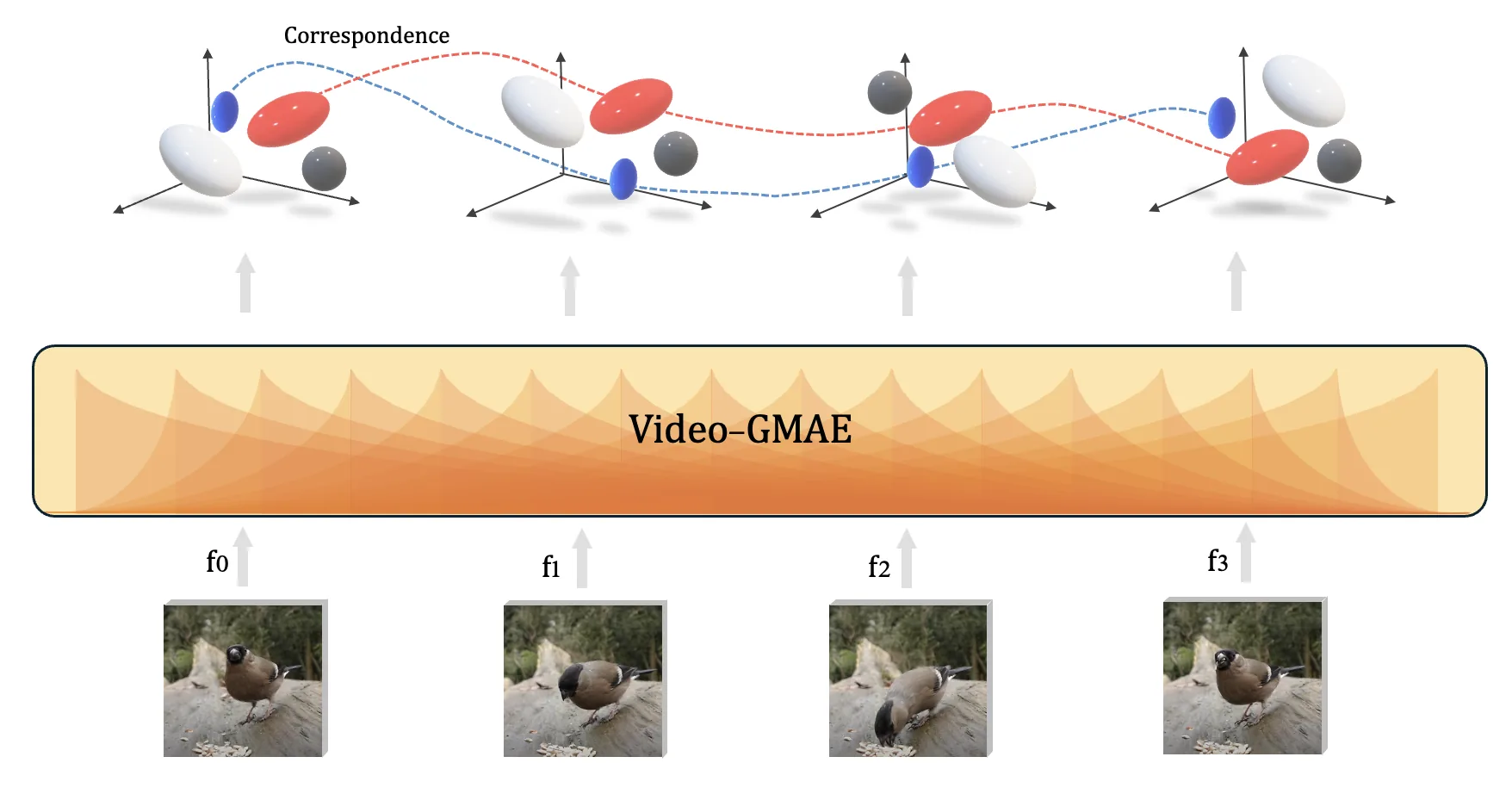
Correspondence emerges directly from the moving Gaussians. The tracker below uses no tracking labels.

DAVIS zero-shot: animals, crowds, vehicles, and occlusions.

Kinetics zero-shot: everyday action clips with varied motion.

Failure cases: camera motion and fine detail can stress the Gaussian budget.

05 Comparisons

Video-GMAE vs. GMRW-C

Video-GMAE is more temporally stable in many clips; GMRW-C can better preserve tiny, fast details.

TAP-Vid Kinetics comparison.

TAP-Vid DAVIS comparison.

06 Fine-tuning

Fine-tuned point tracks

Tuning on labeled tracks from Kubric improves tracking further.

Fine-tuned: TAP-Vid DAVIS, two looped sequences.

Fine-tuned: TAP-Vid Kinetics, two looped sequences.

07 Reconstructions

Pretraining renders

Rendered Gaussian trajectories during pretraining capture coarse structure and motion; fine detail is limited by the 256-Gaussian budget.

Dynamic reconstruction from Gaussians.

08 Benchmarks

Zero-shot and fine-tuned results

Reading motion straight off the Gaussians tops prior SSL trackers; Kubric labels lift the readout into supervised tracker range.

AJ ↑ · no labels	Prior SSL	Ours	Δ OA
Kubric	54.2	54.3	+9.3
DAVIS	41.8	41.3	+6.9
Kinetics	46.9	60.1	+8.9

Zero-shot 60.1 AJ on Kinetics with no trained tracking readout.

Frozen encoder, Kinetics AJ · supervised readout

MAE-ST42.3

VideoMAE46.9

Video-GMAE65.1

Fine-tuned Reaches 74.0 / 75.1 AJ on Kubric / Kinetics, matching state-of-the-art supervised trackers.

09 Limits

Where it breaks

Static-camera assumptions in pretraining can hurt videos with strong camera motion.
The 256-Gaussian budget limits fine-detail fidelity in busy scenes.
Longer-frame correspondence regularization can degrade learning on very long horizons.

10 Citation

BibTeX

@InProceedings{Baranwal_2026_CVPR,
  author    = {Baranwal, Tanish and Singh, Himanshu Gaurav and Rajasegaran, Jathushan and Malik, Jitendra},
  title     = {Tracking by Predicting 3-D Gaussians Over Time},
  booktitle = {Proceedings of the IEEE/CVF Conference on Computer Vision and Pattern Recognition (CVPR)},
  month     = {June},
  year      = {2026},
  pages     = {42527-42537}
}